Webster Cash, Ann Shipley, Steve Osterman and Marshall Joy

An essential step in establishing the viability of x-ray interferometry as a discipline for astronomy is the demonstration of a practical x-ray interferometer. The interferometer must not only create fringes, but be of a design class that can be developed into an efficient system for astronomy.

There have been very few x-ray interferometers successfully built. While there is no question that x-rays will exhibit the same wave properties that light exhibits in other bands, the extreme shortness of the waves has made development of a practical interferometer very difficult. In 1932, Kellstrom used a Lloyd’s Mirror geometry to create x-ray fringes (Nova Acta So. Sci. Upsala, vol 8, 60). This setup, while creating fringes and demonstrating the principle, is extremely inefficient in collecting area, requiring the mirror to operate at a vanishingly small graze angle (i.e. below one arcminute). In 1965 Bonse and Hart (App. Phys Lett, Vol 6, 155) showed that one could use a chain of Bragg crystals to create x-ray fringes. Because of the extreme inefficiency of Bragg crystals, this class of interferometer would be incapable of observing faint celestial sources.

We have now built and successfully tested an x-ray interferometer of a class that can have practical applications. In this section we describe the experiment and show the results.

The instrument is of the simple four flat mirror design shown schematically in Figure 1 below. The work was performed in a 120 meter long vacuum facility at the Marshall Space Flight Center. We used a Manson electron impact source with a magnesium target and 2 micron aluminum filter to create a beam that consists mostly of the Mg K line (1.25keV). The beam passed through a 5 micron exit slit

.

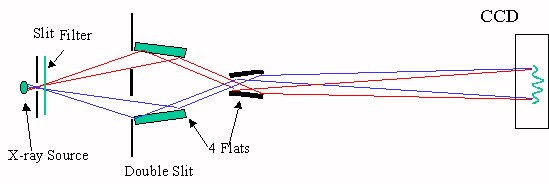
Figure 1: Schematic of Setup

Sixteen meters from the slit the divergent beam entered the interferometer. An entrance aperture that consisted of two parallel slits ensured that the two primary mirrors were illuminated, but that none of the direct beam could enter the interferometer without reflecting off the optics. After passing the double slit, the wavefronts reflected on the primary mirrors. Each mirror was a 50mm circular optical flat mounted at about 0.25 degrees to the incoming beam. Each was mounted in a precision manipulator that allowed fine rotational and translation adjustment from outside the vacuum tank as shown in Figure 2. They were set 0.769mm apart at the front and 0.551mm apart at the back. The primary mirrors created reflected wavefronts that crossed and were then reflected by the secondary mirror.

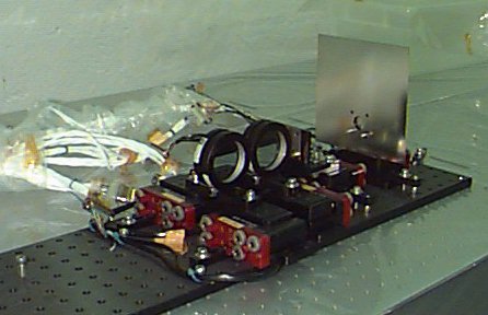
Figure 2: Picture of the interferometer.

The front of the secondary mirrors was 16.97mm beyond the back of the primaries. These mirrors were also 50mm diameter circular optical flats mounted on manipulators. They were set 0.40mm apart at the front, and 0.618mm apart at the back. The wavefronts, when they emerged from the secondary mirrors, were very nearly parallel. They then traveled 100 meters down the vacuum pipe where they were detected by a CCD. The CCD had 18m pixels, was liquid nitrogen cooled, and operated in an individual photon detection mode.

When the system was turned on, each of the two beams created a vertical stripe of illumination on the CCD about a millimeter wide. The final step was to fine adjust the angles of the secondary mirrors so that the two stripes fell on top of each other at the CCD.

On the first attempt (March 8, 1999) we found that one of the channels was too wide on the detector. We eventually tracked this to a mirror that had shifted in its mount during shipping, and had become slightly warped. We returned to Colorado, reseated the mirrors and then returned to Marshall Space Flight Center

.                   

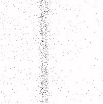
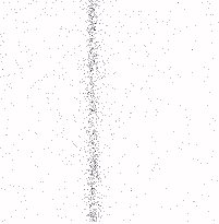
Figure 3: CCD images. Left, before the beams are steered over each other. Right, after alignment, the image contains fringes.

On the second attempt we were successful. Figure 3 shows an image of the CCD with the stripe of illumination clearly visible. Within the stripe of illumination are the fringes we were seeking. When the illuminated region is collapsed into a histogram of events across the x direction, we find the result in Figure 4. The histogram is for the upper half of the CCD only. A two bin boxcar smooth has been run across the data to suppress the Poisson noise.

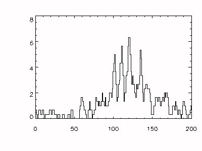
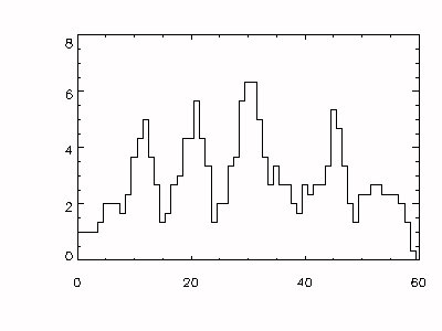
Figure 4: Left, the histogram of counts across the illuminated region. Right, an expansion of the main fringes to show the binning.

Further analysis of the images show that the fringes are not completely well behaved. In Figure 4 one can see that the fringe on the right is a little bit farther apart than the others. This is the result of a 25nm deviation from flat in one of the mirrors near its edge. There are other deviations from flatness in the mirrors that lead to fringes that are not perfectly straight and parallel. This is not a surprise as we are using "l /20" flats from a catalogue. We set the mirrors at 0.25 degrees partly to suppress the surface irregularities.

With this first system we were able to accomplish our goal, to create fringes in an optical setup that is appropriate for development into a full-fledged astronomical system. The sensitivity of the fringes in this setup indicated we achieved sensitivity to angular scales near 0.05 arcseconds.

However, with this initial success comes the question of what to do next. Several things are evident.

1. Straighter Fringes: The mirrors we used were of marginal quality, what would be called l /20 in an optics catalogue. To create well behaved fringes, we should upgrade the optical flats and their holders into the l /100 class.
2. More Compact: We deliberately chose an initial configuration that requires the minimum number of optical elements and the simplest alignment sequence. However, the system had a distance of 100meters between optic and detector. To make the systems more practical and useful, we need to switch to configurations that require only a few meters of length.
3. True Imaging: So far we have only achieved fringe creation. The real goal is to create images from the interferometric information. This needs to be demonstrated.
4. Higher Resolution: Once control of the images is achieved, we need to explore higher resolution systems. This simply requires that the primary mirrors be moved further apart. However, it also requires that the calibration system be properly matched to the system. Smaller slits and more stable pointing are required.
5. Two Dimensional Version: We have recognized that it is possible to phase an array of flat mirrors and achieve imaging that resembles that of a telescope in two dimensions. This should be demonstrated and tested at some point.
6. Spacecraft: As we learn more about the optics and the available design choices, we should continue to investigate their implications for spacecraft design in search of the most practical overall missions.