[ed note: For some reason, this paper is one of my most popular items. If some one of you out there has linked it in some prominent place, would you drop me a line?]
Acoustic Applications of Phased Array Technology
Charles W. Danforth
Johns Hopkins University
January 26, 1998
Updated and reformatted April 5, 2000 by popular request
 Get this paper in PDF format. Get this paper in PDF format.
Abstract:
The angular resolution (beam width) of a detector is proportional to the wavelength divided by the aperture diameter. Hence, for longer wavelengths, a different technology must be used for higher resolution. Phased arrays synthesize larger apertures from an array of elements. The basic theory is explained with 2-element arrays and then expanded with an N-element linear array. Beam-steering and nulling are briefly discussed. This technology is widely used in radar and radio-astronomy, however, in this paper, I present a number of acoustic applications of phased arrays including side-scan sonar, passive sea floor detectors, and towed arrays.
Keywords: Phased Arrays, Sonar, Beam forming, Acoustic Technology
|
|
Optical telescopes yield beautiful, crisp images for one basic reason; the wavelength of light they deal with is tiny compared to the diameter of the aperture it must pass through (the main lens/mirror of the device). However, when longer wavelengths are used, resolution becomes increasingly worse. The angular resolution  is written

where D is the diameter of the aperture and  is the wavelength of light being considered. The 1.22 factor arises from the circular aperture and will be explained shortly.
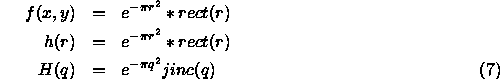
If we consider a point source represented by a Dirac delta function  (x,y) and view it through an circular aperture of radius a, f(x,y), the observed pattern will be the square of the Hankel transform of the convolution of the source and aperture functions or
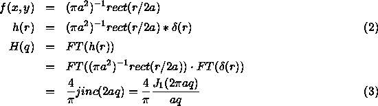
The observed intensity at the detector is then (H(q))2 as represented in figure 1. The location of the first minimum is  0.61 from the axis, half the 1.22 seen in Eq. 1. This is the beam width so important for radio astronomy, radar, sonar, and other applications. Notice that the strength of the side lobes decreases with angle.
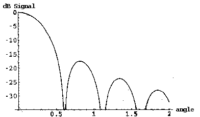
Figure 1: Aperture function from a uniform pinhole.
From Eq. 1, we see that optical images with one arc-second resolution/beam width are possible using a 10cm perfect telescope. However, for the same resolution with microwaves, would require a telescope 250 meters across, something very difficult to engineer. There is a better way to improve resolution.
Phased arrays get around the beam width limit by using several small apertures to achieve the same result as one large aperture. The most dramatic example of this may be the Very Long Baseline Interferometer, a series of 25m radio telescope spaced all over the earth operating at radio wavelengths. By themselves they sport mediocre beam widths insufficient for scientific studies. But when linked together as an array the size of earth, they have a beam width of milliarcseconds, far better than any current optical instrument.
Before we explore the workings of a phased array, it should be noted that the equations and science here makes no distinction between receiving and transmitting devices. For instance, radio telescopes can operate to detect signals from the sky or to broadcast terrestrial messages. While the mechanics of the actual transmitters and receivers may differ, the science here is the same.
Figure 2: Power patterns from a two-element array. Broadside (a), endfire (b), arbitrary phase (c), full-wavelength spacing (d).
Let us examine the simplest case of a 2-element array. Assume we are dealing with devices much smaller than the wavelength of interest and that each broadcasts isotropically. Let us also assume that all measurements are made in the far-field. The power radiated at a given angular position is the square of the sum of the fields put out by the two elements.
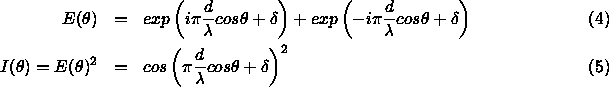
where is the viewing angle with respect to the array axis, d is the separation between the array elements, and is the relative phase of the two emitters. Equation 4 generates an intensity pattern with two lobes, the main lobe and back lobe. By varying the element separation and phase, a number of interesting patterns can be produced (figure 2). The case where the main lobe projects perpendicular to the line between the elements is known as broadside whereas the on-axis case is referred to as end fire. It should be noted that the beam produced by a linear array (of which two elements is the simplest case) is a conical one. The actual radiation pattern in 3-dimensional space is the solid of rotation.
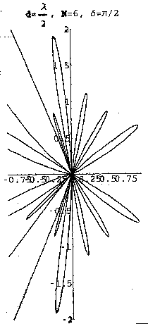
Figure 3: Power pattern from a 7-element evenly spaced, unshaded array set at phase  .
.
Now let's generalize to a linear array of N elements all spaced  apart. (Figure 3) One way to quantify this array is as a series of 2-element arrays (1,2)+(1,3)+...+(1,N) and sum the output (Kraus 1988).

With N=2, Eq. 6 reduces to Eq. 4. The more elements used, the sharper the main beam and back lobe will be. The usual games may be played with the array spacing.
Extending the above analysis to multi-dimensional arrays is simple in concept. While a linear array produces a narrow fan beam of radiation, a plane array can be created to emit a thin pencil beam.
In practice, arrays are often placed in more complicated arrangements. Arrays may be multi-dimensional. Some may feature irregular element separation. The mathematics for arbitrary arrangements becomes complicated quickly and won't be dealt with here. Suffice it to say that with careful numerical modeling, arrays can be designed to fulfill a wide variety of purposes. Upcoming sections will focus on some applications of acoustic arrays.
Recalling the Fourier approach used above, recall that we used a ``square'' aperture with equal transmission at all points with some circle for our calculations. If instead the transmission varied over the surface of the aperture, the Fourier transform, and hence the shape of the beam would be different.
Several outcomes can be obtained by skillful aperture shading. First let's examine an aperture where the transmission is ``shaded'' by a Gaussian function.
This pattern has about the same beam width as that seen in Eq. 2. The one striking difference is that the side lobes are roughly 16 decibels lower. Secondly, let's examine an aperture shaded such that it becomes a narrow annulus.
This main beam is only 2/3 the width of the unshaded aperture but the main lobe is a full 10 decibels lower while the side lobes remain more or less unaffected. (Figure 4).
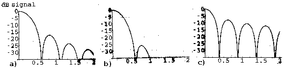
Figure 4: Power patterns for unshaded aperture (a), Gaussian shaded aperture (b), annulus shaded aperture (c).
Applying this technique to phased arrays involves simply giving more or less weight to individual elements. In applications where there is plenty of signal and better resolution or lower side lobes are required, shading may be a good option.
Notice that by changing in Eq. 6, the main lobe and backlobe both shift one direction or the other (figures 2, 3). This represents one of the most significant advances over fixed detectors: fast beam steering. With a single dish antenna, to change the direction, motors and mechanical devices must physically turn the hardware. With arrays, the same effect can be gotten by changing the relative phases of the different elements. This results in a lighter structure with nearly response time limited by electronic rather than mechanical factors.
The downside is that adjusting the phases is nearly always more difficult than rotating the detector. The methods of phase adjustment vary depending on the medium and the frequency being used. Optical devices can be phase-delayed by using mechanical or electronic delay lines or by passing the beams through regions of adjustable index of refraction. Acoustic devices and some lower frequency electromagnetic devices operate at low enough frequency that each element can be individually driven and the phases adjusted by software.
In all previous examples, all array elements have had a consistant phase relationship with their neighbors. However, just as shading offers many options in beamforming, null steering allows sources of noise to be filtered out. The principle of null steering is that the beam is shaped such that a source of noise coincides with a direction of very low power/sensitivity in the beam. The full-blown mechanics of detailed beamforming is beyond the scope of this paper, however, a simple example of null steering presented by Lombardo et.al. (1993) may be illustrative.
In their experiment, Lombardo et.al. (1993) used an acoustic twin-line towed sonar array. It was composed of two 5km strings of hydrophones separated by a distance comparable to the wavelength of the energy being studied (the low frequency sounds of submarines, in this case). With the large number of elements in each string, the mainlobe was quite sharp and could be pointed by either steering the towing ship or adjusting the phases. Unfortunately, a source located in the left beam was indistinguishable from that in the right beam.
To solve this left-right ambiguity, the line separation distance was adjusted such that  . Signals arriving from the right would reach the left line a time
  out of phase with the right line. Signals arriving from the left would reach the left line
  out of phase with those from the right. When the phase is added to the data from the left line, the mainlobe will be brought into phase, while the backlobe data will sum to zero. There is slight degredation in the mainlobe strength, but the backlobe drops to -100dB (Figure 5).
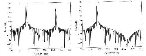
Figure 5: An example of nulling. Before: main lobe and back lobe are of comparable strength. After: back lobe drops by 100dB. (Lombardo et. al. 1993)
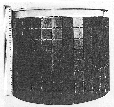
Figure 6: A cylindrical, 192 element echo ranging array. Circa 1980's. The unit is 0.9 meters tall. (Urick 1983) |
The basic sonar system is fairly straight forward. A projector is used to emit a pulse of sound energy. The accoustic waves travel outward and rebound to varying degrees from objects in the field. The reflected wave is then picked up by a hydrophone. Modern sonar systems use piezo-electric or magnetostrictive components both to produce the ping and measure the very small pressure variations associated with the return. They can be manufactured in many ways, but most are made from relatively cheap ceramic materials (Urick, 1983). This is refered to as active sonar. Passive sonar is simply the receiving half of the active system. Figure 6 shows a modern acoustic array.
Even from a very simple one-component echo sounder system such as this, a number of data can be found. From the time delay between transmission and detection, the distance to the reflecting object (henceforth the target) can be found given the velocity of sound in the medium (more on this later). The frequency shift of the returned signal can be used to determine the radial velocity of the target. Thirdly, the strength of the returned signal can help guess the properties of the target. Larger cross-sections will yeild larger returns, however, different materials will reflect differently. Orientation of target surfaces also matter.
One ``feature'' of unique to sonar applications is the high variability of sound speed in a medium. In water, the primary arena for sonar, the sound propagation speed is a function of temperature, pressure and chemical composition (in this case, salinity) (Coates, 1989). Thus in a real body of water, the speed profile varies with seasonal changes and currents. A typical deep-water profile is shown in figure 7a.
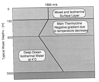
Figure 7a: Sound speed in ocean water (Coates 89).
A consequence of this feature is that sound rays (the path locally normal to the wave fronts) will refract and bend with depth. In the limit where the water depth is small compared to the horizontal distance, grazing rays will reflect and refract. This phenomenon can be exploited in several ways. Rays from a source located in the surface layer (down to perhaps 100 meters) will refract downward into the deep water whereupon they will be refocussed upward. These convergence zones form concentric rings around the horizontal location of the source (Lombardo et. al. 1993) (Figure 7b). Hydrophones placed on the surface at these regions will hear a much stronger signal than those placed in the ``dead zones'' between.
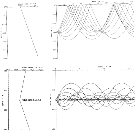
Figure 7b,c: Ray traces of sound above and below the thermocline (Coates 1989).
For sources at greater depth, upward-heading rays may refract downward and never actually reach the surface (figure 7c). Military submarines utilize this phenomenon by cruising below the thermocline, the depth where the sound speed reaches a minimum, thus hiding their acoustic trace from surface ships. Sub-hunting surface craft counter this by deploying deep-running passive arrays (Lombardo et.al. 1993) or by using data from sea-bed arrays (Davis et.al. 1997).
Sonar technology and phased array technology can and have been quite successfully merged with very impressive results (Lombardo et.al. 1993; Boyles & Biondo 1993; etc). A few of the multitude of sonar array applications include passive ``listenning'' arrays for subarine detection. Marine biologists use similar arrays in tracking animal life such as whales. Geologists are able to detect submarine movement of magma and seabed materials. Oceanographers make extensive use of both vertical and horizontal seafloor arrays to study surface waves (Davis et.al. 1997), accoustic propagation speed in various shallow-water areas (Boyles & Biondo 1993), high-resolution mapping of the ocean floor, and seasonal temperature changes.
Certainly one of the more profitable areas of underwater acoustics, it is also one with huge numbers of applications. This technology is frequently used by archeologist, geologists, prospectors and developers, not to mention search-and-rescue teams and practically anyone else who wants to explore the sea-floor. Indeed, high quality side-scan units are commercially available now for a modest price to practically anyone.
The typical side-scan sonar is a short array (typically 50 wavelengths long) encased in a towfish, a torpedo-shaped object towed underwater behind a ship. It typically operates in the hundreds of kilohertz range providing good azimuthal and range measurements. The high frequency limits it to operating in fairly shallow water (a hundred meters). (Figure 8)
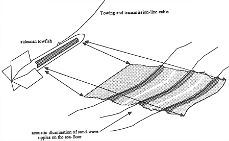
Figure 8: Side-scan sonar system. The towfish is typically a meter or so long (Coates 1989).
As the towfish is pulled through the water, it emits a sonar pulse in a fan-pattern covering a line of seabed. The strength of the return plotted against the delay can then be interpretted as a the illumination of a source as a function of distance. Subsequent pulses give the next lines in what soon becomes a 3-dimensional image. While this data seems very arcane, it is a representation the human brain is extremely good at interpretting. Strong signals belie something strongly ``illuminated'' while areas of little or no signal are ``shadows''. Figures 9 and 10 show particularly stunning samples of these images.
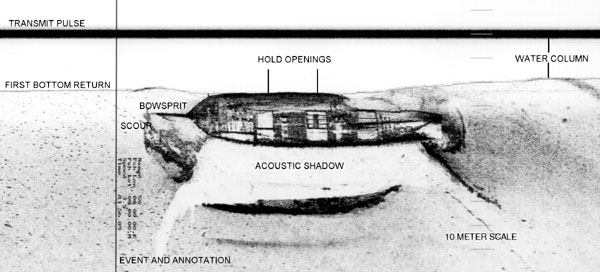
Figure 9: Side-scan sonar image of a wreck (KleinSonar, 1997).
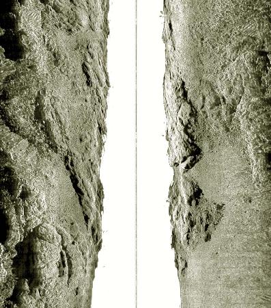
Figure 10: Side-scan sonar image of seafloor geology (KleinSonar, 1997).
The world's naval industries are constantly engaged in a race to make their submarines stealthier and develop better methods of detecting enemy vessels.
Davis et.al. (1997) advanced the cause by using a passive, two-dimensional array layed on the ocean floor connected by fiberoptics to a central telemetry station. This device successfully measured ambient sound in the frequency range 0.01 to 6000 Hz and detected passing ships. Similar arrays feature the ability to monitor surface waves height (the height variation of the water causes pressure fluctuations in the depths) and to monitor local marine life.
A different approach to the same challenge was developed by Lombardo et.al. (1993) with their twin-line towed array. Described more fully in section 2.7, this 5km twin-line array was towed behind a ship in the deep waters south of Hawaii. Using careful beamsteering and nulling (figure 5), they were able to scan the acoustic environment and resolve individual surface ships many hundreds of kilometers distant.
It is no surprise that practically all acoustic arrays operate underwater. There are several reasons for this. Gasses are not good conductors of acoustic energy unlike denser media. The temperature variations in the air are more extreme and faster varying than those in water leading to less well understood refraction systems. Finally, other sensing systems, such as radar and simple visual observation, can operate in air while they are hampered in marine environments.
An interesting non-marine application of passive accoustic arrays is found in a series of military listening posts scattered across the American Southwest (Hoffman 1996). Originally intended to detect the extremely low freqency accoustic (infrasound) signatures of atomic weapon tests, it has proven useful in tracking large meteorites entering Earth's atmosphere.
I am grateful to Dr. Ron Allen of Space Telescope Science Institute, Dr. H. Harold Heaton of the JHU Applied Physics Lab, and Tom Danforth formerly of the Woods Hole Oceanographic Institute for research material, technical discussion and clarification during this project. This project was undertaken as the final exam/project for Ron Allen's Fourier Optics and Interferometry class at JHU and was modified into it's current format due to the surprising response from the public.
References
Boyles & Biondo 1993, ``Modeling Acoustic Propagation and Scattering in Littoral Areas'', JHUAPL Technical Digest, 14, April-June, 162-173
Coates, R.F.W. 1989, ``Underwater Acoustic Systems'', John Wiley & Sons, Inc, New York
Davis, Kirkendall, Dandridge & Kersey 1997, ``64 Channel All Optical Deployable Acoustic Array'', 12th International Conference on Optical Fiber Sensors, Vol 1b, OSA Technical Digest Series, Washington, DC.
Hoffman, I. 1996, ``Scientist Predicts Meteor Collision'', The Albuquerque Journal, December 19
Klein Sonar Systems, http://www.kleinsonar.com, purveyors of fine commercial sonar arrays.
Kraus, J.D. 1988, ``Antennas'', McGraw Hill, New York
Lombardo, Newhall & Feuillet 1993, JHU APL Technical Digest, 14 April-June, 154-161.
Silver, S. (ed) 1949, ``Microwave Antenna Theory and Design'', Dover
Wheeler, Gershon J. 1967, ``Radar Fundamentals'', Prentice Hall
Urick, Robert J. 1983, ``Principles of Underwater Sound, 3rd Ed.'', McGraw-Hill
Charles Danforth
Thursday, November 30, 2000